Exploding Array Function

original Array Notation by Jonathan Bowers
comments and algorithms by Giga Gerard

How it Started

Over the years, I have been interested in large numbers, even to the point of coining names for several, see my "illion numbers" page. One day (about 20 years ago) I read a book (don't remember the name) which discussed operators beyond powers, operators such as tetration, pentation, hexation, etc. This got me interested in investigating more extreme numbers as well as extreme spaces beyond dimensional space (spaces that I now call, super dimensional, trimensional, quadramentional, etc). As time went on, I started to develop an extention to the operators seen in that book, these I will refer to as extended operators. Later after looking into known large number functions such as Ackermann's Function and Conway's Chained Arrow Notation, I could compare the extended operators with these well known functions. The extended operators far surpassed Ackermann's Function, and could actually be compared to Conway's Chained Arrow - check out M. Rob's large numbers page for details. Later I took on the task of extending the extended operators - I later discovered that extended operators could be defined by four numbers, and the next extention by five. This is the beginning of the development of my Array Notation.

Array Notation First row, first dimension in Bean or Beaf

Rule 1: Condition - only 1 or 2 entries - {a} = a, {a,b} = a+b Chris Bird has suggested changing this to a^b for two reasons - first, so it can be easier to compare with Conway's Chained Arrow, second so it will jibe with rule 2 better (note that a^1=a where a+1 is not), I decided to make the change.

Rule 2: Condition - last entry is 1 - {a,b,c,...,k,1} = {a,b,c,...,k}

Rule 3: Condition - 2nd entry is 1 - {a,1,c,d,..,k} = a

Rule 4: Condition - 3rd entry is 1 - {a,b,1,..,1,d,e,..,k} = {a,a,a,..,{a,b-1,1,..,1,d,e,..,k},d-1,e,..,k} - the ".." between the 1's represent 1's - there can be any number of ones, from 1 "1" (3rd entry alone) to a string of 1s - the last 1 of this string is what becomes {a,b-1,1,..,1,d,e,..,k} all entries prior becomes "a". For an array like this {3,2,1,1,1,5,1,2} the last 1 in the string is the one before the 5 (not the one after - since it is a different string of 1s).

Rule 5: Condition - Rules 1-4 doesn't apply - {a,b,c,d,...,k} = {a,{a,b-1,c,d,...,k},c-1,d,..,k}

Extended Operators Sidestep operator notation

a {c} b = {a,b,c}, where c=1,2,3,4,5 etc represents adding, multiplying, exponentiation, tetration, pentation, etc. (After Bird's suggestion, I decided to let a {1} b = a^b instead of a+b to match the modified array notation, so the results are different now).

Tetration is also known as power towers, it is also represented as a^^b = a {4} b (under old version) = a {2} b (under new version) = a^(a^(a^(a^.....^a)...)) a to the power of itself b times.

Pentation is a tetrated to itself b times = a^^^b = a{5}b (old version) = a(3)b (new version), from now on lets use the new version.

Now for the extended operators.

a {{1}} b = a { a { a....a { a { a } a } a.... a } a } a (b a's from center out) - I call this a expanded to b

a {{2}} b = a expanded to itself b times (or a multiexpanded to b) = a {{1}} (a {{1}} (a {{1}} (a .... (b times)

a {{3}} b = a multiexpanded to itself b times (or a powerexpanded to b)

a {{4}} b = a powerexpanded to itself b times (or a expandotetrated to b)

etc.

Evaluate, with reps :n: of words selected by dots to both sides:

{a,b1,1,2} = {a,a,{a,b,1,2}}

          == {a,a,..1.} :b1:

           = {a,a,..a.} :b: = a{{1}}b1

{a,b1,2,2} = {a,{a,b,1,2},1,2}

          == {a,..1.,1,2} :b1:

           = {a,..a.,1,2} :b: = a{{2}}b1

{a,b1,c1,2} = {a,{a,b,c1,2},c,2}

           == {a,..1.,c,2} :b1:

            = {a,..a.,c,2} :b: = a{{c1}}b1

Here's how this compares to Array Notation: a {{c}} b = {a,b,c,2}

a {{{1}}} b = a {{ a {{ a ... a {{ a {{ a }} a }} a ... a }} a }} a ( b a's from center out) - I call this a exploded to b.

a {{{2}}} b = a exploded to itself b times (a multiexploded to b)

a {{{3}}} b = a multiexploded to itself b times (a powerexploded to b)

a {{{4}}} b = a powerexploded to itself b times (a explodotetrated to b)

etc.

Again, here it is compared with Array Notation: a {{{c}}} b = {a,b,c,3} etc.

{a,b,1,3} == {a,a,..1.,2} :b: = a{{{1}}}b

{a,b,2,3} == {a,..1.,1,3} :b: = a{{{2}}}b

{a,b,c1,3} == {a,..1.,c,3} :b: = a{{{c1}}}b

{a,b,c1,4} == {a,..1.,c,4} :b: = a{{{{c1}}}}b

These operators can be notated more naturally:

{a,b,c,5} = a{{{{{c}}}}}b = a{c,5}b

{a,b,c,d} = a{..c.}b {:d:} = a{c,d}b

a {{{{1}}}} b = a detonated to b = {a,b,1,4}

a {{{{{1}}}}} b = a pentonated to b = {a,b,1,5}

{a,b,1,1,2} = {a,a,a,{a,b-1,1,1,2}} = a {{{{{{{....{{{a}}}....}}}}}}} (where there are a {{{{{...{{a}}...}}}}} a brackets (where there are a {{{{..{{a}}..}}}} a brackets ( where there are .......b times ..... (where there are a brackets)))))) - YIKES!!

Chris Bird has shown in a proof (which we can call Bird's proof) that four entry arrays are comparible to Conway's Chained Arrow Notation and five entry arrays far surpass it.

No real difference between operators and array function here.

{a,b,1,1,2} = {a,a,a,..1.} :b: = a{1,1,2}b

{a,b,2,1,2} = {a,..1.,1,1,2} :b: = a{2,1,2}b

{a,b,c1,1,2} = {a,..1.,c,1,2} :b: = a{c1,1,2}b

{a,b,1,2,2} = {a,a,..1.,1,2} :b: = a{1,2,2}b

{a,b,c,2,2} = a{c,2,2}b

{a,b,c,d,e} = a{c,d,e}b

{a,b,c,d,e,f,g,h} = a{c,d,e,f,g,h}b

{a,b,Z} = a{Z}b

Currently I have operator notations for up to 8 entry arrays (i.e. {a,b,c,d,e,f,g,h}), however they will be quite cumbersome to type out - a,b, and c are shown in numeric form, d is represented by brackets (as seen above), e is shown by [ ] like brackets, but rotated 90 degrees, where the brackets are above and below (uses e-1 bracket sets), f is shown by drawing f-1 Saturn like rings around it, g is shown by drawing g-1 X-wing brackets around it, while h is shown by sandwiching all this in between h-1 3-D versions of [ ] brackets (above and below) which look like square plates with short side walls facing inwards. - one of these days, I'll add a jpeg.

Extending Array Notation Bean system

Later I decided to extend array notation (which used a 1-D array) to allow for many dimensions in the array - I called it Extended Array Notation. Since multidimensional arrays are difficult to type out, Bird suggested using bracketed numbers to represent separating n-D structures, example: {3,3,3 (1) 3,3,3 (1) 3,3,3 (2) 3,3,3 (1) 3,3,3 (1) 3,3,3 (2) 3,3,3 (1) 3,3,3 (1) 3,3,3} represents a 3-D array - a 3^3 array of 3's to be exact, which when solved will give the enormous number "dimentri".

Following are the rules for Extended Array Notation using Bird's inline technique:

Rule 1: Condition - only 1 or 2 entries, only 1 dimension - {a} = a, {a,b} = a^b was originally a+b

Rule 2: Condition - rows ending with 1. - {# (n) a,b,c,...,k,1 (m)#} = {# (n) a,b,c,...,k (m) #} - # denotes remainder of array.

Rule 3: Condition - 2nd entry of main row (which is the very first row) is 1 - {a,1,c,d,..,k #} = a

Rule 4: Condition - 3rd entry is 1, next non-1 entry in same line - {a,b,1,..,1,d,e,..,k #} = {a,a,a,..,{a,b-1,1,..,1,d,e,..,k #},d-1,e,..,k #}

Rule 5: Condition - Rules 1-4 doesn't apply, there are at least 3 entries on main row - {a,b,c,d,...,k #} = {a,{a,b-1,c,d,...,k #},c-1,d,..,k #}

Rule 6: Condition - two entries on main row, next non-1 entry begins a row - (a,b (n)...(k) c #} = {b^n array of a's (n)...(k) c-1 #} - this is hard to describe, but the (n)...(k) could be anything from going to the next row (i.e. (1)) to something like this: (4)(4)(4)(4)(4)(3)(3)(3)(3)(2)(2)(2)(2)(2)(2)(2)(2) - which means going into the next 5 4-D regions, then into the next 4 realms (3-D), then into the next 8 planes - this example will be solved as {b^4 array of a's (4) b^4 array of a's (4) b^4 array of a's (4) b^4 array of a's (4) b^4 array of a's (4) b^3 array of a's (3) b^3 array of a's (3) b^3 array of a's (3) b^3 array of a's (3) b^2 array of a's (2) b^2 array of a's (2) b^2 array of a's (2) b^2 array of a's (2) b^2 array of a's (2) b^2 array of a's (2) b^2 array of a's (2) b^2 array of a's (2) c-1 #}.

Rule 7: Condition - two entries on main row, next non-1 entry is preceded by 1's in it's row - {a,b (n) ... (k) 1,1,...1,1,c #} = {b^n array of a's (n) ... (k) a,a,...a{a,b-1 (n) ... (k) 1,1,...1,1,c #},c-1 #} - same thing with the (n) ... (k)

As you can see - the rules are getting very complicated to write down

Yet one can keep going into higher spaces, higher than dimensional space - consider the tetrational spaces (which includes super dimensions, trimensions, quadramensions, etc.) - what is this exactly - dimensional spaces can be represented as X^n R^n = {a,b,[n]2} where X represents a line, X^2 would then be a plane, X^100 would be 100 dimensional. Super dimensions are of this order - X^(X^n), trimensions, quadramensions, etc are as follows: X^(X^(X^n)), X^(X^(X^(X^n))), etc. - these kind of arrays are possible - so array notation can be addapted to these arrays, but the rules get trickier. Using Bird's inline technique we can represent super dimensional space as follows: {# (a,b,c,....,k) #} which represents going to the next a'th dimension of the b'th second level of dimensions of the c'th third level of dimensions .... of the k'th n'th level of dimensions - notice this is only super dimensions, it gets crazier in trimensions on up.

Let schematic expressions X^Y denote dimensional structures.

{3,2,[1,2]2} = D[3,2,1,2]

             = D[3,3,3] = {3,3,[3]2}

             = D[3,3,2],[2]D[3,3,2],[2]D[3,3,2] = R^3

Superdimensional Bean:

{a,2,[1,2]2} = D[a,2,1,2] = D[a,a,a] = R^a

{a,3,[1,2]2} = D[a,3,1,2] = D[a,a,{D[a,a,a]}] = R^R^a

{a,b,[1,2]2} = D[a,b,1,2] = R^^b

{a,3,2,[1,2]2} = {a,{a,a,[1,2]2},[1,2]2} = R^^R^^a

Super-pentational Bean: 

{a,b,2,[1,2]2} = R^^^b 

{a,2,c,[1,2]2} = R^..a ^:c

{a,b,c,[1,2]2} = R^..b ^:c1

But Arrays can go even further - there are also pentational arrays such as an X^^^6 array which would be an X^^(X^^(X^^(X^^(X^^X)))) array where X^^X alone would be an X^(X^(X^(....^(X^X))....)))) array. Bird has attempted to write rules for extending past dimensional arrays and appears to have captured rules that fit tetration and possibly pentation - but they get quite tedious.

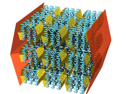
Below is a picture showing a 2 superdimensional array that leads to the number "dulatri" - the yellow brackets represent dimensional groups - inside could take on any number of dimensions, they represent X^X structures, the red brackets represents an X^X array of X^X arrays - or an X^(2X) array.

Exploding Array Function Beaf principles

Definitions:

Array - a structured set of entries (the array will be represented as A)

Entry - a position in the array that holds a positive integer value (1 is default - so any entry not represented automatically has the value of 1)

Base - first entry (value represented by b)

Prime entry - second entry (value represented by p)

Pilot - first non-1 entry after prime entry (can be as early as 3rd entry, can be in a different dimension or beyond)

Copilot - entry right before pilot (if pilot is the first entry on its row, then there's no copilot. Copilot might be the prime entry itself, if the pilot is 3rd entry.

Structures - structures are sub-arrays of the following types: entry (X^0), row (X^1), plane (X^2), realm (X^3), flune (X^4),..,X^n,..,dimensional group (X^X)=X^^2,..,n-D array of dimensional groups (X^(X+n)),..dimensional group of dimensional groups (X^(2X)),...X^(2X+n),...m-D array of dim.group of dim.group of.....dim.groups n times (X^(nX+m)),...dimensional gang (X^(X^2)),...X^(polynomial),...X^(X^X)=X^^3,....X^(X^X+polynomial),........X^^4,....X^^n,...X^^X,......X^^^X,....X^^^^````^^^X,...etc.

Previous Structures - previous entries are entries before the pilot but are on the same row, previous rows are rows before the pilot's row, but are in the same plane, previous n-spaces are n-spaces in the same n+1-space that are before the pilot's n-space, etc. They are structures before the pilot's version of that structure, but on the same structure that is of higher order.

Prime Block - the prime block of an X^n structure is the first p^n block of entries left of an n-dimensional separator (n) in that structure, - this generalizes to all structures, turning the X's to p's, where p is the prime. - so if p=10, and the structure is X^(3X^5+2X^4+3X+6), the prime block is exploded to the first 10^(3*10^5+2*10^4+3*10+6) set of entries.

Airplane - a set of entries that include the pilot, all previous entries, and the prime block of all previous structures.

Passengers - any entry in the airplane that is not the pilot or copilot. This will always include the base.

Allowance: Default entries (entries that have a 1 value) can be chopped off as long as none of the entries change their positions.

Rules:

Rule 1 - the prime rule - Condition: default prime (p = 1) - Result: v(A)=b. where v(A) means value of array.

Rule 2 - the initial rule - Condition: no pilot - Result: v(A)=b^p.

Rule 3 - the catastrophic rule - Condition: first two rules don't apply - Result: Array changes in the following way:

1. pilot decreases by 1.
2. copilot (if exists) becomes original array, but with its prime entry reduced by 1.
3. (*Prime Blocks of) Previous Structures X^n are exploded to sizes p^n & b values, so all passengers take on base value.
4. remainder of array remains unchanged.

That's it!! - much simpler - and even more powerful, in that it can be continued as long as the structures can be defined.

Notational rule 0 - finalize trailing entries - Allowance to drop any default (dead) and last (right) entries with value 1 together with their preceding (left) separator if it is trailing too. This is not strictly necessary (for further evaluation), but cleans up the expression.
Provided the signifying (highest) right separator of (*the Prime Block of) every Previous Structure remains, we can choose to drop the default entries with their (lower) left separators, because rule 3c (or 3c*) will overwrite all defaulted substructures with sizes very much larger than the current ones.
A left separator (n) of an entry 1 is considered "trailing" (and redundant), when it has a larger (*or equal) separator (m) directly on the right.

The difference in rule 3c - between exploding only the Prime Blocks (3c*) of Previous Structures, or keeping and exploding all Previous Structures up to the pilot entry - is often negligible. When higher separators occur further on the right (past the pilot) this rule difference is provably insignificant for the resulting Big numbers. The development of higher structures dominates the algorithm.
Nevertheless we feel that keeping all separators signifying Previous Structures (*not just Prime Blocks) in rule 3c would be the natural method for Beaf. Natural, because Bowers allows multiple b,p (n).. (n):m to explode to m series of (n) separated structures of sizes p^n & b values. This is pretty obviously maximal, when applied to the explosion of run down Previous Structures.

Types of Arrays

Linear:

Linear arrays consists of one row, ex: {3,5,6,1,3,4,2} - these are the smallest and simplest arrays - even though the arrays are small, the value of the arrays can be so huge that not even Conway's Chained Arrow notation can keep up (an array with only 5 entries will clobber Chained Arrow!!). The positions on the array can be represented by a positive integer, i.e. the 17th position.

Dimensional:

Dimensional arrays have a multidimensional structure - these are the second smallest arrays. These arrays consists of rows, planes, realms, flunes (4-spaces), and various n-spaces. The rules above can easily handle dimensional arrays - although the results seem to nearly reach infinity. The positions in the array can be described with a linear array, i.e. (4,5,3,1,2) represents the 4th entry on 5th row on 3rd plane on 1st realm on 2nd flune. Dimensional arrays can be represented as follows: {4,2,5,7 (2) 5,6,1,2 (2) 5,4 (1) 6 (3)(3)(2) 2,5,6 (1) 1,1,1,7 (2) 6,8,5,2 (5) 7,5,6,8}. Here (2) represents going to next second dimension (or going to next plane), (3) is next realm, (5) is next 5-space.

Tetrational:

These arrays go way beyond dimensional arrays, and take on structures that require tetrational spaces. They consist not only of rows, planes, realms, etc, but also dimensional groups, rows of groups, planes of groups, groups of groups, groups of groups of groups of groups, gangs, rows of gangs, groups of gangs, gangs of gangs, realms of groups of groups of gangs of gangs of gangs, etc, etc, etc, superdimensional groups, trimensional groups, etc,etc. These are the third smallest arrays (and the largest type that I have fully grasped how they work). Tetrational arrays consist of super dimensional arrays, trimensional, quadramensional, etc in the same way dimensional arrays consists of planar, realmic, flunic, etc arrays.

Positions of superdimensional arrays can be described by a dimensional array, i.e. (5,6,3 (1) 3, 5 (1) 6,7 (2) 5) represents the 5th entry of the 6th row of the 3rd plane of the 3rd dimensional group, of the 5th row of groups, of the 6th group of groups, of the 7th row of group of groups of the 5th dimensional gang. To represent a 3^(3^2) array, let A represent the 3^3 dimensional group {3,3,3 (1) 3,3,3 (1) 3,3,3 (2) 3,3,3 (1) 3,3,3 (1) 3,3,3 (2) 3,3,3 (1) 3,3,3 (1) 3,3,3}, now a 3^(3^2) array of 3's would be {A,A,A (1,1) A,A,A (1,1) A,A,A (2,1) A,A,A (1,1) A,A,A (1,1) A,A,A (2,1) A,A,A (1,1) A,A,A (1,1) A,A,A} To get a 3^(3^3) array let A be equal to the group of groups mentioned above (the 3^(3^2) array that is) and let (1,1) and (2,1) change into (1,2) and (2,2) respectively.

Positions of trimensional arrays can be described by a superdimensional array, positions of a quadramensional array can be described by a trimensional array, etc.

Pentational:

Next in line are pentational arrays, these require pentational spaces. Trying to understand how these work might give someone a migrane. One would need to keep up with tetration levels which can also get out of hand. There will be tetrational groups that show up here, X^^X arrays are more tidy examples of tetrational groups. a X^X^X^X^X array is a tetrational one, quintamensional to be exact (keep in mind that powers are solved in reverse) - for pentational arrays, the powers will sort into groups, i.e. an X^X^X^X^{X^X^X^X^X}^{X^X^X^X^X}^{{X^X^X^X^X}^{X^X^X^X^X}^{X^X^X^X^X}^{X^X^X^X^X}^{X^X^X^X^X}} array, the {} are not to be solved like ordinary parenthesis, but are used to group up the exponents into tetrational blocks - the number of entries in this array can be found out by removing the {} and solving - ie. X^^39 in this case - and this is barely scratching the beginning of pentationals.

Beyond Pentationals:

Hexational, heptational, expandal, multiexpandal, explosal, powerexplosal arrays, etc. arrays so huge that the space its in needs to be represented by array notation (linear, dimensional, tetrational, and so forth) - how to work with these? - Only God knows - but they should form some massive arrays - and utterly unspeakable numbers when solved.

After superdimensions come the Next Legion arrays:

{3,3,1,2,[1,2]2} = {3,3,{v},[1,2]2} = 3^..3 ^:v

    v = 3,2,1,2,[1,2]2 = 3,3,3,[1,2]2 = 3^^^^3 

{a,3,1,2,[1,2]2} = a^..a ^:v ≅ a1&a&a&a

    v = a,a,a,[1,2]2 = a^..a ^:a1 ≅ a1&a&a

Bowers devises new notations for old style recursions: 

a,b1,1,2,[1,2]2 = {a,a,..a.,[1,2]2} :b:

    ≅ a1.&a.. :b1 ~ {a1,b2 /2} = Â

Big boowa example:

3,3,3 /2 =

  3,v,2 /2 = 3,..1. /2 :v:

    v = 3,2,3 /2 = 3,3,2 /2 = 3,3&3&3 /2  <~

3,3,3,2,[1,2]2 =

  3,v',2,2,[1,2]2 = 3,..1.,1,2,[1,2]2 :v':

    v' = 3,2,3,2,[1,2]2 = 3,3,2,2,[1,2]2

       = 3,{3,3,{3,3,3,[1,2]2},[1,2]2},1,2,[1,2]2

Bowers' 2nd legion defined on the row:

a,b,c,2,[1,2]2 ≅ {a,b,c /2}

a,b,c,d1,[1,2]2 ≅ {a,b,c,d /2}

a,b,c,d1,R,[1,2]2 ≅ {a,b,c,d,R /2}

Structures preceding the 3d legion:

a,2,[1,2]3 = D[a,a,a],[1,2]2 = a^a /2

a,b,[1,2]3 = D[a,b,1,2],[1,2]2 = a^^b /2

a,3,2,[1,2]3 = a,{a,a,[1,2]3},[1,2]3 = a^^^3 /2

a,b,c,[1,2]3 = a^..b /2 ^:c1 ≅ c1&b&a /2

Next legions defined on the row: 

a,b,1,2,[1,2]f1 ≅ {a1.&a.. /f} :b ~ {a,b1 /f1}

a,b,c,1R,[1,2]f ≅ {a,b,c,R /f}

The Next Legion:

Let & represent "array of", so 3 & 3 = {3,3,3} = tritri = 3 to the power of itself 3^27 times - now consider 3&3&3 (solved frontwards) this is a {3,3,3} array of 3's which is a 3^^^3 array of 3's - now imagine a new array notation such that the second rule changes to this:

Condition - no pilot, result - v(A)=b&b&b&b&.....&b&b -- p times - welcome to the next level of array notation.

Another way to represent this is to simply add an entry with value 2 in a second "legion", where the first legion can take on any of the previous arrays - {3,3 / 2} = 3&3&3, the big boowa = {3,3,3 / 2} = 3&3&3&3&3&............&3 - where there are 3&3&3.......&3 3's arrayed to each other - where there are 3&3&3.....3 3's arrayed to each other - where there are 3&3&3.....&3 3's arrayed to each other - ... - ... - ... - - - - this is said 3&3&3&3&......&3 times - where there are 3&3&3 3's arrayed to each other here before getting to the end (which is "where there are 3 3's arrayed to each other")!!! - keep in mind that in {3,3,3 / 2} 3,3,3 are in the first legion and 2 is in the second legion - this 2 represents "second level of array notation".

One can consider {b,p / 2} as if the pilot is in the 2nd legion, and in this case the airplane is defined to be a b&b&b...&b p times - array in the first legion - of course you can go to the 75th level of array notation if you like - {b,p / 75} = {b&b&b....&b - p times - array / 74}. Note that {A / 1} = A, so 1's are still default.

Linear Legion Arrays:

{A1 / A2 / A3 / A4 / ..... An} - here each of the An's are arrays (can be linear, dimensional, tetrational, pentational, etc - up to but not including legion arrays) - nuf said!!!

Linear legion arrays resolved from right to left:

D[a,b,c],[1,2]f  = Â /f

a,b,1,2,[1,2]2,2 == a,v,[1,2]1,2  with v = Â

     = D[a,v,1,2],[1,2]{a,v-,[1,2]1,2}

    == D[a,v,1,2],[1,2]{..1.} :v:

     = R^^v,[1,2]{..a.} :v:

     = Â,[1,2]{..a.} :v:

     = Â /..a #Â ~ Â(/2)Â = Â(/3)2

Arrays of Bean translated to Bowers' dimensional legions:

a,b,2,2,[1,2]2,2 = Â(/2)Â(/2)Â = Â(/3)3

a,b,c,2,[1,2]2,2 = Â(/3)c1

a,2,1,3,[1,2]2,2 = a,a,a,2,[1,2]2,2 = Â(/3)a1

a,3,1,3,[1,2]2,2 = Â(/3)Â(/3)a1 ~ Â(/4)3

a,b,1,3,[1,2]2,2 = Â(/4)b

a,b,2,3,[1,2]2,2 = Â(/5)b

a,b,c,3,[1,2]2,2 = Â(/c3)b

Further array structures are ill-defined, we imagine that:

a,b,R,[1,2]2,2 = Â(/R)b

a,b,[1,2]3,2 = Â(/Â)b ~ Â//2 (Legion legions)

a,b,R,[1,2]3,2 = Â(/Â)Â(/R)b

a,b,[1,2]c1,2 = Â//c ~ Â(//2)2

a,b,[1,2]c,3 = Â///c ~ Â(///2)2

a,b,[1,2]c,d = Â/..c /:d

a,b,[1,2]c,d,2 = Â/../(1)c /:d

a,b,[1,2]c,d,e1 = Â/../(1)..c /:d /(1):e ~ Â/(2)e

a,b,[1,2]ci,..z ci,:n ~ Â/(n)z 

a,b,[1,2],[1,2]2 ~ Â/(Â)b ≅ L (Legion space) 

Dimensional Legions, Tetrational Legions, Legion Legions, and beyond:

One can take arrays further to include things like the following:

{A / A / A / A (/2) A / A / A (/3,4,5,2) A } - this is a tetrational legion array.

{3,3 // 2} - a legion legion array - this is equal to 3&&3&&3, where 3&&3 = {A / A / A} where A = 3&3&3 array (in other words 3&&3 is a 3 legion array of 3's), 3&&3&&3 = 3&&3 legion-array of 3's. - note that a mere 3^3 legion array of 3's would be {A / A / A (/1) A / A / A (/1) A / A / A (/2) A / A / A (/1) A / A / A (/1) A / A / A (/2) A / A / A (/1) A / A / A (/1) A / A / A} - which is nothing compared to a 3&&3 legion array of 3's

{3,3 /// 3} - a legion legion legion array - which equals 3&&&3&&&3, where 3&&&3 = {A // A // A} where A = 3&&3&&3 array of 3's

{3,3 //////////////// 2 } - use your imagination.

{3,3 ///(1)///(1)///(2)///(1)///(1)///(2)///(1)///(1)/// 2 } - the next step would be to give the legions themselves an added structure - {3,3 (1)/ 2} (the legion mark is in the second row of legion marks) - but how would we define this, first lets come up with a new kind of space called "legion space" - we can think of it as the highest extent of space before we encounter the legions, in the same way that X represents the line, and X^X is above all dimensional space, legion space "L" is above all of the non-legion array notation spaces - that means it is beyond tetration {X,n,2}, pentational {X,n,3}, linear array-spaces {X,X,X,X,X,X,...,X}, dimensional array-space 100^100 & X's, and even X&X&X&X&X&5 - the prime block of a legion space would be b&b&b&b....&b - p times (b=base). Legion of legions describe the double legion marks //, while a legion "of itself" 50 times would have 50 legion marks - so lets define {L,n}_b,p as legion of legion of legion of....legion - n times using b and p as the base and prime. {L,1}_b,p = {b,p / 2} = b&b&b&b&b... p times, {L,2}_b,p = {b,p // 2} = b&&b&&b&&b... p times - which is the prime block of a legion of legions. {L,X}_b,p = {b,p (1)/ 2} = {b,p //////....///// 2} - p /'s - notice how the previous row of /'s is the prime block of the row of /'s - so we can still use that rule here. Next we can do {L,A} - where A is an array-space - this will lead to the legion marks themselves taking on an array structure, not just the separate legions. We can continue with {L,L} - here the legion marks will take on legion space - and it gets worse, for {L,L} = {L,2,2}, so lets go for {L,3,2} - this would be {L,{L,2,2},1} = {L,{L,L}} - the legion marks taking on a legion of legions - can you feel the tension. Next would come things like {L,X,2}, {L,A,2}, {L,X,6}, {L,L,L,L,L,L,L,L}, 100^100 array of L's - this is array notation on the legion space - all this will lead to the next group - "lugions"

In Bowers' gallery of numbers a Mark Lugo steals the show:

a,b,ci..,[1,2],[1,2]2  ,ci:n  ≅ {L,..1} L,:n2

a,b,[1,2],[1,2]3  ≅ L2

a,b,[1,2],[1,2]n1  ≅ Ln

Approximately Bowers' last batch:

a,b,[1,2],[1,2],[1,2]2  ≅ LL

a,b.,[1,2]..2  :n1  ≅ L.. :n

a,b,[2,2]2  ≅ M 

A plausible upper bound to Bowers' final fantasy: 

a,b,[13,5,2]2  ≅ MEA!

a,20,[1,[1]2]2 ~> MEAMEAMEALOKKAPOOWA!

10,20,[15,15,13,16,2,[1]2]2 ~>

  MEAMEAMEALOKKAPOOWA OOMPA! < 3,3,[3,[1]3]3

Lugions, Lagions, Ligions, and beyond

We will use the following to describe lugions, the lugion mark is \, "legiattic array of" mark is @ (symbols were suggested by John Spencer), and finally Lugion space will be L2. {L2,1} _b,p = {b,p \ 2} = b@b@b@b....@b - p times - where n@m = {L,L,L,.....,L}_n,m - there are m L's - so a 3@3 legiattic array is {L,L,L}_3,3 - a 3@3@3 legiattic array would be {L,..a....,L}_3,3 where a = {L,L,L}_3,3. We can continue with double lugions (or lugions of lugions) {L2,2} cases which lead to double lugion marks in the arrays "\\". Look what can be done to the lugiattic space arrays - {L2,X}, {L2,A}, {L2,L}, {L2,B} - B is a legiattic array, {L2,L2} = {L2,2,2}, {L2,L2,L2,L2,L2,L2}, 100^100 array of L2's, legiattic array of L2's - and finally the lagions L3 - we can do similar things there. Lagion marks are |'s, we can use % to denote "lugiattic array of". L4 space is the ligion space, we can use "-" for ligion marks, and # for "lagiattic array of". Of course we can continue to L5,L6,...L100,...L(gongulus),......

Going even further

Now imagine LX space where the X can change to p when finding the prime blocks of the space, L(X+1), L(2X), L(X^2), LA, LL, LL2, LLL, LLLLLLLLLLL, LLLL(1)LLLL(1)LLLL (3 rows of L's) - 10^100 array of L's (no comma's between them this time) - just use the imagination to where this could lead . . . MEAMEAMEALOKKAPOOWA OOMPA!

Beate is the acronym for the algorithm Beate's Express Array Train Extra

and its rules are discussed above as a variation on our definition of Beaf,

with series of the (accumulated) b uploaded left of V (instead of items a).



Inspired upon our restoration of the ancient Indian Asamkhyeya

– the incalculable number 10^(5*2^104) (a tower of squares).



    Beate's Mountain Top =

    10,5,[.. .]2  :104:  in Beate  ,[ ] ≡ ,



Algorithmically larger than the highest of Bowers' numbers, but still below infinity

– for a higher type of countable infinity, replace the coefficients above by omega ω.